LAB 2 Acceleration of Gravity

                                 Lab 2 ACCELERATION OF GRAVITY


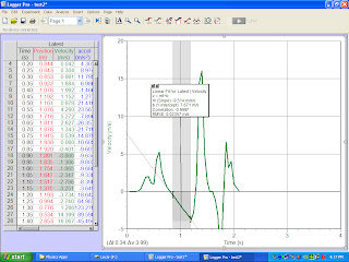
Purpuse of graph : To determin the acceleration for a freely falling object.
                          : To gain experience in the computer as a data collection.

Object : ball

Equipment Used : windows based computer, Lab pro interface,Logger Pro software,motion detector,rubber ball,wire basker.

What we did: Loaded logger pro software on the position vs time graph. We changed the verical scale from 0 to 4 m and the horizontal scale or time to 0 to 4 seconds.  We placed the motion detector on the floor facing upward and placed wire basket over the detector. After setting up the motion detecor we started the testing. Giving the ball a toss up about 1 meter above the detector.  After a few tosses we obtained a graph with a parabol showing the balls motion going up and down. Graph located in Ex: 1. We then selected the ata in the interval that corresponds to the free falling motion of the ball. Then we choose analyze/curve fit from the menu at the top of the menu. We selected  at²+bt+c (quadratic) and then selected Try Fit   obtaning the values for a,b,and c. To find the acceleration,gexp, of the ball from this data and to calculate the precent diffrence between the value obtained and the one accepted value,gecc,(9.80m/s²) we did the following equations

At²+Bt+C where A=( value obtain from table)

        ( 1/2) *(g)where g=9.80

we obtained the % error using the following equation

Percent = (measured-actual/measured) x100% 

liner fit = mt+b
                                   UNIT ANALYSIS
G expected = (2(4.9071m/s^(2)))= 9.814 m/s^(2)

% difference = ((9.814m/s^(2)-9.800m/s^(2))/9.800m/s^(2))x(100%)=.1429%

G expected(m)=-9.500m/s^(2) from graph

% difference=((9.500m/s^(2)-9.800m/s^(2))/(9.80m/s^(2))x(100%)= -3.060%
                                  DIMENSIONAL ANALYSIS
G expected= 2(m/s^(2))= x m/s^(2)

%difference=( [m/s^(2)-m/s^(2)]/[m/s^(2)])*100%= x%

G expected(m)= m/s^(2) from graph

%difference= ([m/s^(2)- m/s^(2)]/m/s^(2))100% =  x%

The following are the graphs that we made based on the 5 trials made: 

                              VELOCITY VS. TIME

1ST

2ND

Here is are result tabel for the fallowing 5 trials.

Reslults from From Falling Body Experiment
Trials	gexp(2a)(m/s^(2))		%diff	gexp(m)(m/s^(2))		%diff
1	9.814  m/s^(2)		0.143	9.5	m/s^(2)	3.06
2	9.612  m/s^(2)		2.04	9.514	m/s^(2)	2.917
3	9.860 m/s^(2)		0.61	9.528	m/s^(2)	2.78
4	9.541 m/s^(2)		2.65	9.497	m/s^(2)	2.24
5	9.170 m/s^(2)		6.42	9.532	m/s^(2)	2.73

The 5 graphs for positon vs time.
                                            POSITION VS TIME

1ST

2ND

My conclusion is that based on the graphs including Velocity vs. Time and Position vs.Time and are calculaions shown on the table. Given the gravity was 9.80 m/s^(2) and most of are calculation wher 0.3 to 0.2 off are graph show a accurate representaio of the ball in freefall motion. And because the velocity is equal to the gravity becaus there is no other force applied it. And because are experimen show that ar g obtained was on the average 9.500 m/s^(2) are percent diffrence was 2%. Becasue of this we obtained the results expected for the acceleratin for a free folling object in are graphs. 

Graphical Analysis

BY:JOVANY CRUZ

                                        FIRST LAB GRAPHICAL ANALYSIS
In this lab the purpose was to gain experience in drawing graphs and in using graphing software. In part 1 we learned how to use the Graphical Analysis software. We learned how to open and use funcion plot graph and how to make a function and graph it . We learned how to add a title to the function and labelthe  x & y axis and how to add units. This is a example of are funcion and the graph that goes with it.

For the part 2

we connected the lab pro to the computer and motion detector to DIG/SONIC2 port to the lab pro. And we opend the mechanics folder and open the graphlab file. And then we practice recording position vs. time graph. After a few trial of dropping the the ball to record the motion we got a nice curve. We then selected the appropriate datar range and performed a fit to the data. It had the general quadratic form of At^2+Bt+C where A=-4.469,B=4.980,C=1.210. Yes in part the acceleration is due to gravity. What is n in the equation

UNIT ANALYSIS: dαg(t)ⁿ

S²m=m/S²(S)ⁿxS²

S²=Sⁿ

N=2
 DIMENSIONAL ANALYSIS:   
dαg(t)ⁿ
[l ]α[l/t^(2)] [t^n]

So n=2 in the equatuion . we finally used dimensional anaysis and unit analysis to verify the equation. Here is a picture of are equation.

Conclusion: we learned how to use the graphical analysis software for the very first time. And selected a function "x2"sin(3^(x)x2") for are graph. We also learned that n=2 in the following equation dαg(t)^(n).