Lab 4 Vector Addition of Forces

Vector Addition of Forces

Purpose: The purpose of this lab was to study vector addition by:

1.    Graphical means

2.    Using components

3.    Using a circular force table to check results

Equipment:   -Circular force table                 -Masses

                       -Mass holders                    -String

                      -Protractor                          -Four pulleys

Procedure used:

1.    We were given three masses in grams as well as three angles as shown in figure 1. And obtained a scale of 1cm=20grams and made a vector diagram showing these forces, and graphically fond the resultant. We determined the magnitude (length) and direction (angle) of the resultant force using a ruler and protractor as shown in figure 1.  figure 1  
   

     Mass given                    degrees given

          150g                                      0˚

        110g                                       70˚

        250g                                       135˚

We then divided by the ratio given 1cm=20g to get

Grams changed to

 New grams         same degrees

7.5cm                                    0˚

5.5cm                                    70˚

12.5cm                                  135˚

Vector addition and degrees with length from lab are total was 14.0cm. we used tan^(-1)(14.0cm/0.54cm)=87.79 degree are new degree.

2.    Made a second vector diagram that showed the same three forces again. Found the resulting vector again, by components as shown in figure 2. We also showed the components of each vector as we as the resultant vector on are diagram as shown below.figure 2 we used tan^(-1)(14.0cm/0.54cm)=87.79 degree are new degree

3.    We then mounted three pulleys on the edge of our force table at the angles given above. We then attached strings to the center rings so they each run over the pulley so each run over the pulley and attached the mass holder as shown in figure 3A. We then hang the appropriate masses= force in grams on each string. We then set up a fourth pulley and mass holder at 180 degrees opposite from the angle we calculated for resultant of the first three as shown in figure 3a and 3b.  
figure 3a

Diagram showing how we verified the results. figure 3b Shows our mounted pulleys at equilibrium.  And our % error was =0.14% .

4.     

Unit analysis

      

150gx1cm/20g=7.5cm

110gx1cm/20g=5.5cm

250gx1cm/20g=12.5cm

 X Comp=7.5cos (0˚) +5.5cos (70˚) +12.5cos (135˚) =0.54cm

Y comp=7.5sin (0˚) +5.5sin (70˚) +12.5sin (135˚) =14.01cm

V xy=abs((.54)^(2)+(14.01)^(2))^(1/2)=14.02cm

Resulting angle vector. Tan^(-1)(14.02cm/.54cm)= 87.79˚

Dimensional analysis

gx cm/g=cm

g x cm/g=cm

g x cm/g=cm

 X Comp= cos (degrees) + cos (degrees) +  (degrees) = cm

Y comp= sin (degrees) + sin (degrees) + sin (degrees) = cm

V xy=abs((x)^(n)+(x)^(n))^(n)= cm

Resulting angle vector. Tan^(-1)(cm/cm)= degrees

Conclusion

Our conclusion was that the percent error was 0.14% meaning we did things right in our lab. Based also on the scale the middle strings were right on the middle with the ring exactly in the center.  Also it was low because of the fact that we were given 3 vectors and trying to find the 4 vector.  Overall we learned how to add vectors based on their components using the head to tail method.

LAB 3: Acceleration of Gravity on an Incline Plane

       Acceleration of Gravity on an Incline Plane

Purpose: The purpose of this lab was to find the acceleration of gravity by studying the motion of a cart on an incline.

Equipment used:    - windows based computer            - Logger pro software

                                   - Motion detector                               - Ballistic cart

                                   - Aluminum track                                - Wood blocks

                                   - Meter stick                                         - small carpenter level

Quick description:   In this lab we will used the computer to collect position (x) vs. time (t) data for a car accelerating on an inclined track. When comparing acceleration of the car moving up and down friction is eliminated. And we can find the acceleration of gravity only. If g is the acceleration due to gravity when car is in free fall, the acceleration along the track is g sinƟ and Ɵ is the angle of incline for the track.

Procedures we did:

1. connected labpro to the computer as well as the motion detector opened and loaded the Logger pro.

2. Inclined the track slightly by putting the wood friction block under the track approximately at the 50cm mark. Then used a bubble level or small carpenter level to make sure it was leveled from both sides. Then we found out what was the incline angel Ɵ by measuring the vertical and horizontal travel as shown in figure 1 below.
 

figure 1:shows how we solved for  Ɵ  when h=50 cm, x=49.95cm .  cosƟ=49.95cm/50cm  àƟ=cos^(-1)(49.95cm/50cm) àƟ=2.56˚

3. We then placed the detector at the upper end of the track facing down toward the bottom. Then we placed the car at the lower end and gave it a push up hill near the detector brining it no closer than 50cm to it. As shown in figure 2 below.

 figure 2

4. Started taking data on computer after car left hand. Meanwhile  we were observing both the position and the velocity graphs simultaneously. And properly labeld the graphs for position vs. time, velocity vs. time with titles and units etc. as shown in the figure 2 A.

                                                 Trial 1 using 2.56˚ three grpahs

                    

                                                                                                                          graph 1

                     graph 2

grpah 3

figure 2A show all 3 trials for small angle 2.56˚

   

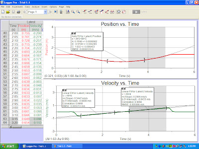
 5.We found the accelerations, a1 and a2, of the car by determining the slope of the v vs. t curve for each portion of the motion going up and down. Then we selected a range  of time that represents the motion going up the incline. Then we selected analyze/curve fit and fit the selected portion to a linear function of time. The slope was the acceleration a1. Then we did the same thing for a2 and used                              g sinƟ= (a1+a2)/2   equation to determine g as in figure 3 A.

figure 3A: we solve for g=([.3447m/s^ (2)+.2995m/s^ (2)]/2)/ sin(2.56˚)=7.212m/s^ (2)

6. We did two more trials for the same incline. We then average are values and calculated are g and compared are results with the accepted value 9.80m/s^(2) as shown in figure 3B.
   figure 3B

                                                            SUMMARY TABLE  1^st trial using Ɵ=2.56˚

g experimental g=([a1+a2]/2)/sin(2.56˚)	Average = (1. +2. +3.)/3	Actual g=9.80 m/s^(2)	% difference = ([Experimental-actual]/actua)l x100%
1.       7.212 m/s^(2)	Average for	9.80 m/s^(2)	26.4%
2.       7.064 m/s^(2)	All  g experimental=	9.80 m/s^(2)	27.9%
3.       7.101 m/s^(2)	7.125 m/s^(2)	9.80 m/s^(2)	27.5%

7. We repeated experiment (steps 2, 5 and 6) for the larger angle 5.73˚ by using larger block of wood to increase the angle of inclination of the track. As shown in figure 4A-figure  below.                
                                           Experiment 2 Larger angle

 

figure 4A :shows how we solved for  Ɵ  when h=50 cm, x=49.75 .  cosƟ=(49.75cm/5ocm)  àƟ=cos^(-1)(49.75cm/50cm) àƟ=5.73˚.

 figure 4B: For motion sensor setup we then placed the detector at the upper end of the track facing down toward the bottom. Then we placed the car at the lower end and gave it a push up hill near the detector brining it no closer than 50cm to it. As shown in picture above.

Figure 4C: shows three graphs for are 2nd experiment with the larger angel. We Included the appropriate labeling s title, and units etc.

 1 graph  2nd graph 3 rd graph

 figure 4D:

We did two more trials for the same incline. We then average are values and calculated are g and compared are results with the accepted value 9.80m/s^(2)

                                                            SUMMARY TABLE  2^st trial using Ɵ=5.73˚

g experimental g=([a1+a2]/2)/sin(5.73˚)	Average = (1. +2. +3.)/3	Actual g=9.80 m/s^(2)	% difference = ([Experimental-actual]/actua)l x100%
1.      1.   7.250 m/s^(2)	Average for	9.80 m/s^(2)	26.00%
2.      2.   7.227 m/s^(2)	All  g experimental=	9.80 m/s^(2)	26.25%
3.      3.   7.252 m/s^(2)	7.243 m/s^(2)	9.80 m/s^(2)	26.00%

  Unit analysis

    we solve for g=([.3447m/s^ (2)+.2995m/s^ (2)]/2)/ sin(2.56˚)=7.212m/s^ (2)

  Solving for Ɵ àƟ=cos^(-1)(49.95cm/50cm) àƟ=2.56˚

Solving for g experimental= ([7.255m/s^(2)+9.80255m/s^(2)]/2)/sin(5.73˚)= 7.250m/s^(2)

Solving for the average      = (2.250 m/s^(2)+7.225 m/s^(2)+7.252 m/s^(2))/3= 7.243 m/s^(2)

Solving %difference          = ( 7.250 m/s^(2)- 9.80 m/s^(2))/( 9.80 m/s^(2))x100%=26.00%

                                                 dimensional analysis

Solving for g experimental= ([m/s^(2)+m/s^(2)]/2)/sin(Ɵ  )=  m/s^(2)

Solving for the average      = ( m/s^(2)+ m/s^(2)+m/s^(2))/3=  m/s^(2)

Solving %difference          = ( m/s^(2)-  m/s^(2))/(  m/s^(2))x100% = %

 we solve for g=([m/s^ (2)+m/s^ (2)]/2)/ sin(Ɵ) = m/s^ (2)

  Solving for Ɵ=cos^(-1)(cm/cm) àƟ = x˚
                                

                                                 Units used in graph in si units

Time = s      Position = m    Velocity = m/s   g= m/s^(2)

                                                Conclusion

Based on the graph on what we talked in class are g experimental was on the average 7.243 m/s^ (2) and the actual g is 9.80 m/s^(2) meaning are percent error was 26% which is a lot. The problem was that are area measured was small therefore increasing are percent error was big. Had we used a larger are we would have a smaller percent error or percent difference as are teacher mentioned in class. But we did find the acceleration of gravity we were looking for.